Objective: Determine whether or not SOI is the best metric to measure El Nino in CESM-WACCM4.

Tasks

1. Calculate Pacific Ocean temperature composite of all months when the SOI less than -1.0 and greater than 1.0.

TS={}; case='nw_ur_150_07'; case = 'control'
#TS[case] = extract_entire_data('TS',files[case])
TS[‘control’] = extract_entire_data('TS',files['control'])
SOI= np.load('/home/josh/Documents/150Tg/NINO_REPORT/SOI_ts.npy').item()
wSOI_months = warm_SOI_months(SOI[case])
cSOI_months = warm_SOI_months(SOI[case],crit_val = 1.0)
wSOI_months_DJF = warm_SOI_months(SOI[case],'DJF')
wSOI_months_JJA = warm_SOI_months(SOI[case],'JJA')
TS_anomaly = monthly_anomaly(TS['control'],TS['control'])
data_NINO = np.nanmean(create_composite(TS_anomaly,wSOI_months),axis=0)

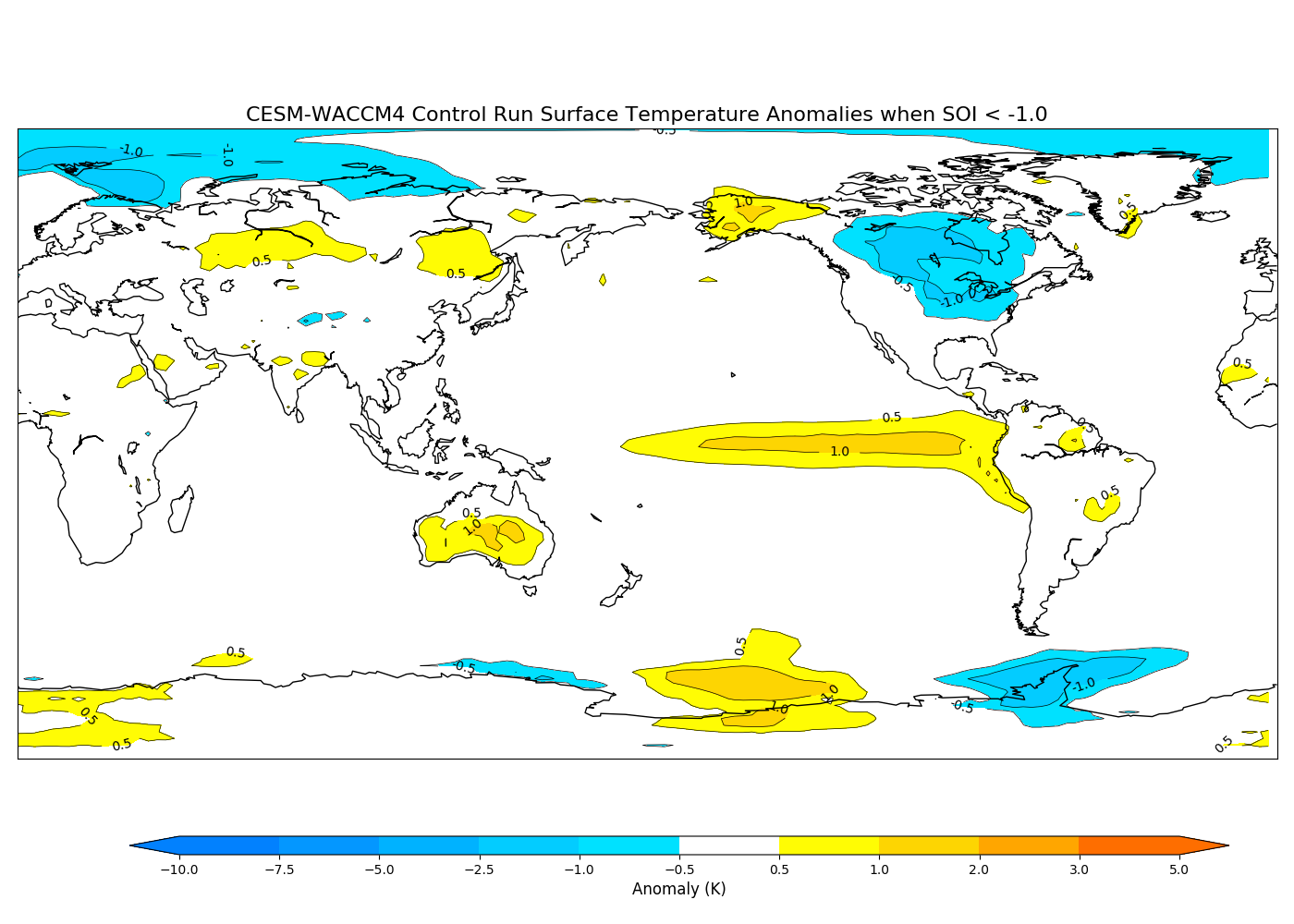
given_title = 'CESM-WACCM4 Control Run Surface Temperature Anomalies when SOI < -1.0';
savefile = '/home/josh/Documents/NW_NINO_PAPER/random_plots/fig.png'
custom_map_quiver(data_NINO,'SST','K',given_title,lat1=-90,lat2=90,lon1=0,lon2=360,scl=100,U='none',V='none')

data_NINA = np.nanmean(create_composite(TS_anomaly,cSOI_months),axis=0)
given_title = 'CESM-WACCM4 Control Run Surface Temperature Anomalies when SOI >1.0';
savefile = '/home/josh/Documents/NW_NINO_PAPER/random_plots/fig.png'
custom_map_quiver(data_NINA,'SST','K',given_title,lat1=-90,lat2=90,lon1=0,lon2=360,scl=100,U='none',V='none')

Clearly, this shows that when the SOI is less than -1.0 (El Nino Conditions, 43 out of 252 months) in CESM-WACCM4, there is strong warming across the central and eastern Pacific Ocean. Additionally, similar cooling occurs when the SOI is greater than 1.0 (La Nina Conditions, 41 out of 252 months).

2. Calculate statistical correlation between Nino 3.4 and SOI during nw_cntrl_03 and during nw_ur_150_07 (use RSSTs).

import numpy as np
from scipy import stats
case = 'control'
SOI= np.load('/home/josh/Documents/150Tg/NINO_REPORT/SOI_ts.npy').item()
wSOI_months = warm_SOI_months(SOI[case])
cSOI_months = warm_SOI_months(SOI[case],crit_val = 1.0)

SST = extract_entire_data('TS',files['control'])
SST_anom = monthly_anomaly(SST,SST); SST34=[]
for t in range(len(SST_anom)):
SST34.append(weighted_meanX(SST_anom[t],lat1=-5,lat2=5,lon1=170,lon2=240))

slope, intercept, r_value, p_value, std_err = stats.linregress(SOI['control'],SST34)

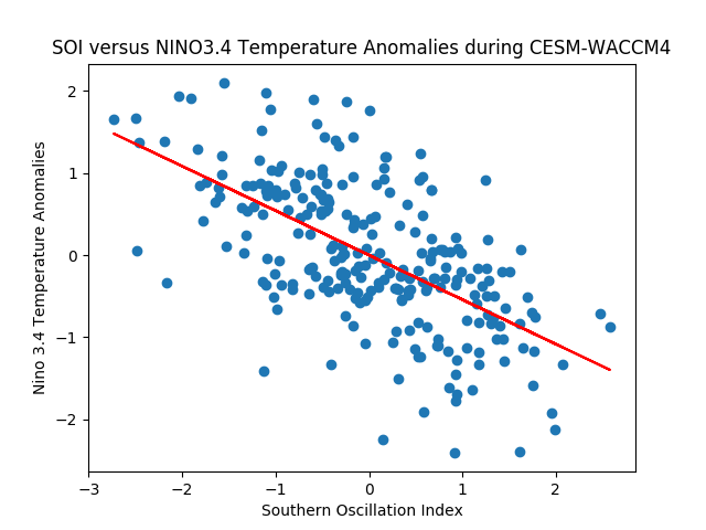
r^2 = 0.61, p = 2e-27 for a linear regression between the Southern Oscillation Index (SOI) and Nino 3.4 temperature anomalies for CESM-WACCM4.

plt.figure()
plt.scatter(SOI['control'],SST34);
plt.plot(SOI['control'],slope*np.array(SOI['control'])+intercept,'r')
plt.xlabel('Southern Oscillation Index'); plt.ylabel('Nino 3.4 Temperature Anomalies');
plt.title('SOI versus NINO3.4 Temperature Anomalies during CESM-WACCM4')
plt.savefig('/home/josh/Documents/NW_NINO_PAPER/random_plots/fig2.png')

Analyze relationship during case = 'nw_ur_150_07' :

case = 'nw_ur_150_07'
SOI= np.load('/home/josh/Documents/150Tg/NINO_REPORT/SOI_ts.npy').item()
#wSOI_months = warm_SOI_months(SOI[case])#
#cSOI_months = warm_SOI_months(SOI[case],crit_val = 1.0)

SST = extract_entire_data('TS',files[case])
SST_control = extract_entire_data('TS',files['control'])
SST_anom = monthly_anomaly(SST,SST_control); SST34=[]
for t in range(len(SST_anom)):
SST34.append(weighted_meanX(SST_anom[t],lat1=-5,lat2=5,lon1=170,lon2=240))

slope, intercept, r_value, p_value, std_err = stats.linregress(SOI[case][0:192],SST34)

r^2 = 0.42, p = 1.78e-9 for a linear regression between the Southern Oscillation Index (SOI) and Nino 3.4 temperature anomalies for CESM-WACCM4 during the nuclear winter run.

plt.figure()
plt.scatter(SOI[case][0:192],SST34);
plt.plot(SOI[case][0:192],slope*np.array(SOI[case][0:192])+intercept,'r')
plt.xlabel('Southern Oscillation Index'); plt.ylabel('Nino 3.4 Temperature Anomalies');
plt.title('SOI versus NINO3.4 Temperature Anomalies CESM-WACCM4'+loading[case])
plt.savefig('/home/josh/Documents/NW_NINO_PAPER/random_plots/fig3.png')

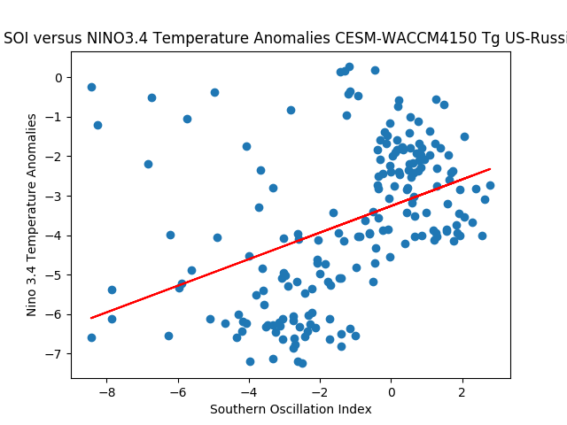
Obviously this is a spurious correlation, as global cooling causes temperatures in the Nino 3.4 region to plummet, while global cooling also causes strong El Nino conditions. Therefore, we must examine RSSTs. Using the methodology from Khodri et al. (2017), the RSST anomaly is defined as the residual signal obtained after removing the mean tropical (20 °N–20 °S) SST anomalies. This allows us to remove the signal of global cooling from a commonly used metric for El Nino, the temperature anomalies in the Nino 3.4 region. Additionally, RSST better characterizes the atmospheric convective response to SST gradients.

RSST34=[]
for t in range(len(SST_anom)):
RSST34.append(weighted_meanX(SST_anom[t],lat1=-5,lat2=5,lon1=170,lon2=240)-weighted_meanX(SST_anom[t],lat1=-20,lat2=20,onlyLand=True))

slope, intercept, r_value, p_value, std_err = stats.linregress(SOI[case][0:192],RSST34)

plt.figure()
plt.scatter(SOI[case][0:192],RSST34);
plt.plot(SOI[case][0:192],slope*np.array(SOI[case][0:192])+intercept,'r')
plt.xlabel('Southern Oscillation Index'); plt.ylabel('Nino 3.4 RSST');
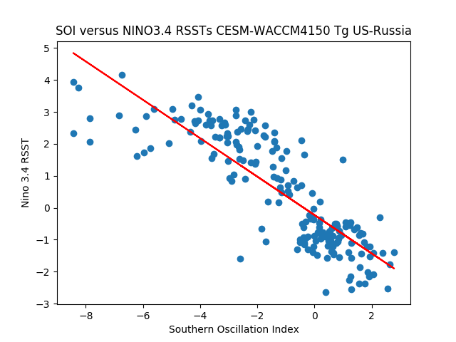
plt.title('SOI versus NINO3.4 RSSTs CESM-WACCM4'+loading[case])
plt.savefig('/home/josh/Documents/NW_NINO_PAPER/random_plots/fig4.png')

r^2 = 0.84, p= 9.5e-52 for a linear regression between the Southern Oscillation Index (SOI) and Nino 3.4 RSST anomalies for CESM-WACCM4 during the nuclear winter run.

3. Examine the literature to determine how well CESM-WACCM4 simulates El Nino.

Reason for concern with previous models - Gabriel and Robock, 2015. Stratospheric geoengineering impacts on El Nino/Southern Oscillation

Main findings: Very little change to frequency or amplitude of ENSO in AGW (RCP 4.5) or stratospheric geoengineering scenarios. ENSO typically exhibits a 2-7 year periodicity with warm (El Nino) and cold (La Nina_ events, each lasting 9-12 months and peaking during DJF. (McPhadden, 2006).
Zebiak and Cane, 1987) – ZC model describes the coupled ocean-atmospheric dynamics of the tropical Pacific.
Emile-Geay et al. (2007) – showed that El Nino events tend to occur in the year subsequent to major tropical eruptions, including Tambora (1815) and Krakatau (1883). Used 200 ZC simulations lasting 1000 years each, showed the probability of an El Nino event in the year after a simulated volcanic forcing never exceeded 43%.

Clemenet et al. (1996) – a uniform solar dimming is likely to result in a muted zonal SST gradient across the equatorial tropical Pacific because the western Pacific mixed layer's heat budget is almost exclusively from solar heating. In the east, both horizontal divergence and strong upwelling contribute to the mixed layer heat budget.
A diminished zonal SST gradient weakens the trade winds and results in less upwelling, an elevated thermocline, leading to the Bjerknes feedback.
La Nina event probability peaks in the third year post-eruption (Maher et al., 2015).
CLIVAR CMIP3/CMIP5 metrics for assessing ENSO: ENSO amplitude, structure, spectrum, and seasonality. Process-based variables, including the Bjerknes feedback were studied.
* 65% of CMIP5 models produce ENSO amplitude within 25% of observations as compared to 50% for CMIP3.
* Bjerknes feedback shows less consistent improvement in CMIP5.
Absence of a shift from a subsidence regime to a convective regime in the eq C Pacific during El Nino.
*this error led to the muting of negative shortwave feedback
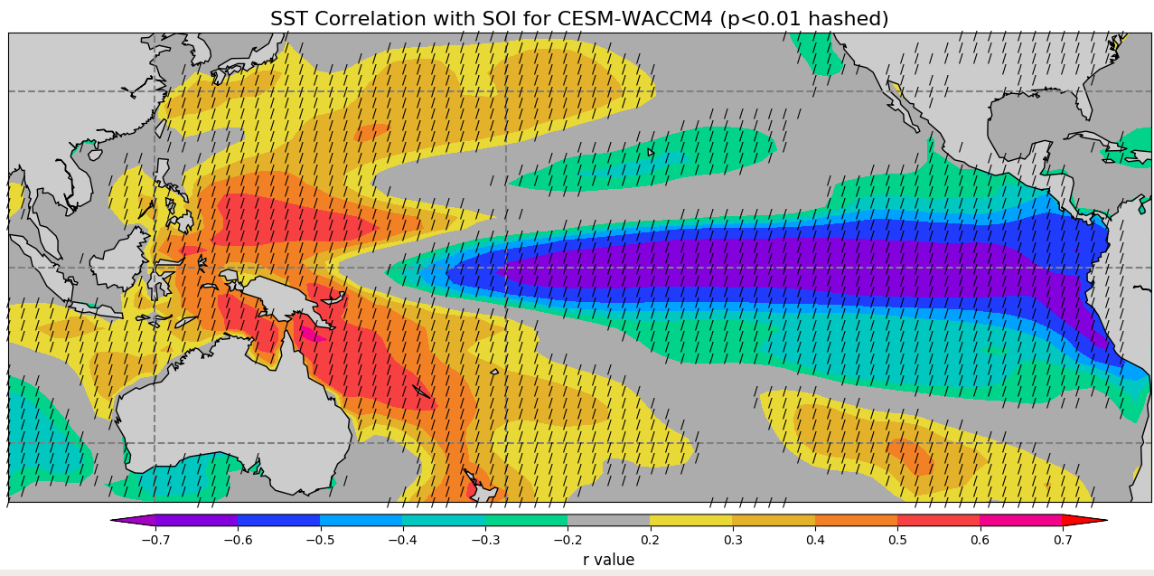
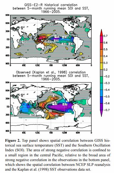
FOR CMIP5 MODELS, SOI simulations show muted variability when compared with SSTs. The area of prominent ENSO variability covers a smaller spatial area than seen in observations.
The maximum values of the SST/SOI correlation in the historical models and observations over same period are approximately the same (r = 0.8).

Task: Create a map that shows the correlation of TS with SOI for the entire Pacific.

import numpy as np
from scipy import stats
case = 'control'
SOI= np.load('/home/josh/Documents/150Tg/NINO_REPORT/SOI_ts.npy').item()
#wSOI_months = warm_SOI_months(SOI[case])#
#cSOI_months = warm_SOI_months(SOI[case],crit_val = 1.0)

SST = extract_entire_data('TS',files[case])
#SST_control = extract_entire_data('TS',files['control'])
SST_anom = np.array(monthly_anomaly(SST,SST));

SOI_SST_corr = np.zeros((96,144))
SOI_SST_pval=np.zeros((96,144))
SST_anom_5mo = running_mean_3darray(SST_anom,2)
for lat in range(96):
for lon in range(144):
slope, intercept, r_value, p_value, std_err=stats.linregress(SOI[case][2:250],SST_anom_5mo[2:250,lat,lon])
SOI_SST_corr[lat][lon] = r_value
SOI_SST_pval[lat][lon] = p_value

from mpl_toolkits.basemap import Basemap, shiftgrid, addcyclic; XYZ='test'

#levels = [-1,-0.8,-0.6,-0.4,-0.2,-0.1,0.1,0.2,0.4,0.6,0.8,1.0];
levels = [-0.7,-0.6,-0.5,-0.4,-0.3,-0.2,0.2,0.3,0.4,0.5,0.6,0.7];
levels_pval=[0.05,0.1]
#colors = get_colors('seismic',len(levels))
colors=('#A203C4','#8201DC','#213BFC','#00A2FF','#00C8C0','#01D38A','#ACACAC','#E9D937','#E4B22A','#F28024','#F64042','#F1028A','#FA0200')
lat1 = -40; lat2 = 40; lon1 = 95; lon2 = 290;
lat1 = -89; lat2=89; lon1=1; lon2=357.5;
map = Basemap(projection='cyl', llcrnrlat=lat1, urcrnrlat=lat2, llcrnrlon=lon1, urcrnrlon=lon2, resolution='c',)
fig1 = plt.figure(figsize = (14,10))
lats = [-90,-60,-30,0,30,60,90]; lons = [-180,-120,-60,0,60,120,180]
for lat in range(len(lats)):
plt.axhline(lats[lat],color='grey',linestyle='--')

for lat in range(len(lons)):
plt.axvline(lons[lat],color='grey',linestyle='--')

latitude,longitude = get_gridding()
yt1,xt1 = np.meshgrid(longitude[:],latitude[:]); y,x = map(yt1,xt1)
SOI_SST_pvalm = maskoceans(y,x,SOI_SST_pval)

#CS = map.contour(y,x,SOI_SST_pval,colors = 'k',levels = levels_pval,linestyles='-',linewidths=0.5)#
#clabels = plt.clabel(CS, inline=True,fontsize = 10, fmt = '%1.2f');
'''
for lat in range(96):
for lon in range(144):
if SOI_SST_pval[lat][lon] < 0.011 and str(SOI_SST_pvalm[lat][lon])=='--':
plt.text(longitude[lon],latitude[lat],'/',horizontalalignment='center',fontsize=10)
'''

CS = map.contour(y,x,SOI_SST_corr,colors='k',levels=levels,linestyles='-',linewidths=0.4)
sc = map.contourf(y,x,SOI_SST_corr, colors=colors, levels = levels,extend='both')
clabels = plt.clabel(CS, inline=True,fontsize = 10, fmt = '%1.1f')
map.drawcoastlines(); map.fillcontinents()
plt.title('SST Correlation with SOI for CESM-WACCM4 (p<0.01 hashed)',fontsize=16)
#plt.yticks([-90,-60,-30,0,30,60,90],('90S','60S','30S','EQ','30N','60N','90N'))#
#plt.xticks([-180,-120,-60,0,60,120,180],('180W','120W','60W','0','60E','120E','180E'))
position = fig1.add_axes([0.10,0.075,0.85,0.02])
cb = fig1.colorbar(sc,cax = position,ticks=levels,orientation='horizontal');
cb.set_label('r value',fontsize=12)
plt.subplots_adjust(hspace = 0.5)
plt.tight_layout(rect=[0, 0.09, 1, 0.95],h_pad=0.5)
plt.show()
plt.close()

Literature on CESM-WACCM4 and El Nino

Rao, J. and Ren, Rongcai, (2016). Asymmetry and nonlinearity of the influence of ENSO on the northern winter stratosphere: 2. Model study with WACCM, J. Geophys Res, 121,9017-9032. doi:10.1002/2015JD024521.

Nonlinearity and assymetry of ENSO events reproduced by CESM-WACCM generally similar to observations, but differences exist. SST anomaly centers in CESM-WACCM extend farther west of the Nino3 region for both El Nino and La Nina. SST anomalies occupy a much narrower band across the equator than observations. Also some differences in the SST anomalies in the tropical Indian Ocean during ENSO (more amplified than they should be , Rao and ren, 2016a).

Marsh, D.R., Mills, M.J., Kinnison, D.E., Lamarque, J., (2013). Climate Change from 1850 to 2005 Simulated in CESM1(WACCM). Journal of Climate, 26, 7372 - ???. doi:/10.1175/JCLI-D-12-00558.1

CESM-WACCM is able to reproduce the periodicity of the Nino 3.4 Index but the amplitude of the signal is somewhat larger. Unsure how this relates to SOI, however. Possibly could be due to addition of turbulent mountain stress (TMS), which was responsible for dramatic improvement in frequency of NH SSWs.

Yun, K-S., S-W. Yeh, and K-J. Ha (2016), Inter-El Niño variability in CMIP5 models: Model deficiencies and future changes, J. Geophys. Res. Atmos., 121, 3894– 3906, doi: 10.1002/2016JD024964.